This handout outlines (through examples) the CS 100 "subset" of MATLAB. The MATLAB help facility should be used for details. The book Getting Started With Matlab by Rudra Pratap is an excellent and inexpensive reference.
One-dimensional arrays are called vectors and two-dimensional arrays are called matrices. Scalars are 1-by-1 matrices. The memory manager takes care of the necessary storage allocations. There are no declarations. The entries in a Matlab array may be real or complex.
When in the command window, you are prompted to enter commands
with a double arrow ">>".
|
|
|
>> x = [ 10 20 30 ]x = 10 20 30 >> x = [10; 20; 30] x = 10 20 30 >> x = [10 20 30;40 50 60] x = 10 20 30 40 50 60 >> x = linspace(1,3,5) x =
u = [1 2]; v = [3 4]; >> x = [u v u] x = 1 2 3 4 1 2 >> x = [u;v;u] x = 1 2 3 4 1 2 >> x = rand(2,3) x = .293029 .343293 .292930 .411275
|
Square brackets delimit
arrays. Row vector entries are separated by blanks.
For columm vector entries are separated by semicolons.
Matrix rows are separated by semicolons.
linspace(a,b,n) sets up
a length-n row vector of equally spaced values from a to b inclusive.
Row vectors can be concatenated to build longer row vectors.
Blanks in between the vectors entries.
Column vectors can be "stacked" to build longer column
vectors. Semicolons in between the vector entries.
rand(n,m) generates an
n-row, m-column matrix of random numbers, each selected from the uniform(0,1)
distribution.
|
| Use help to learn more about linspace, logspace, ones, zeros, rand, and randn. | |
|
|
|
| >> x
= [30 10 80 20 60];
>> n = length(x) n = 5 >> [z,idx] = max(x) z = 80 idx = 3 >> z = sort(x) z = 10 20 30 60 80 >> x = [1 2 3; 4 5 6] x = 1 2 3 4 5 6 >> [m n] = size(x) m = 2 n = 3 |
The length of a vector equals
the number of components.
Use max to find the largest (i.e., most positive) entry
in a vector. Two values are returned. The size of the largest value and
the index that identifies its location. Works for row or column vectors.
Sort sorts the entries in a vector from smallest to largest
(i.e., from most negative to most positive.)
The size of a two-dimensional array isdefined by the number of its rows and the number of its columns. |
| Use help to learn more about length, size, max, min, sum, cumsum, prod, cumprod, sort and median.. Elementary functions like abs, sqrt, exp, log, log10, sin, cos, tan, asin, acos, atan, floor, fix, ceil, round, rem, real, and imag accept array arguments and return the corresponding array of function evaluations. Try help elfun for a synopsis of Matlab's elementary function library. | |
|
|
|
| >>
x
= [5 8 -2];
>> y = [1 2 3]; >> z = x+y z = 6 10 1 >> z = 3*x z = 15 24 -6 >> z = x+7 z = 12 15 5 >> z = x.*y z = 15 16 -6 >> z = x./y z = 5 4 -.66667 >> z = x.^y z = 5 64 -8 >> z = x.^2 z = 25 64 4 >> z = [1 2 3]' z = 1 2 3 |
You can add to vectors as long
as they have the same length and orientation.
This is how you multiply every entry in an array by the same scalar. Componentwise division and exponentiation.
A shortcut for z = x.^[2 2 2].
You can change the orientation of an array this way. Row-vectors
become column-vectors and vice versa.
|
| Array operations for column vectors and matrices are similarly defined. Learn more about array-level operations by typing help ops. | |
|
|
|
| >> x
= pi
x = 3.1416 >> format long >> x = pi x = 3.14159265358979
x = input(`Enter x:'); y = sqrt(x); s = sprintf(`sqrt = %10.6f',y); disp(s) |
The effect of a command is displayed
if there is no semicolon after the command.
The format command is
used to establish the current display style. The short
format (5 decimal places) is in force when Matlab is first entered. The
long
format displays full working precision. Scientific notation is available
via the short e and long
e formats.
To solicit scalar input with a prompt, use input. Disp displays strings and sprintf can be used to produce formatted output strings. %10.6f specifies a decimal format with 6 decimal places and total space allocation of 10 characters. Use e format for scientific notation and d for integers.
|
| Use help to learn more about format, disp, sprintf, input, and num2str. | |
|
|
| Matlab supports matrix-vector multiplication, linear equation solving, data fitting, differential equation solving, nonlinear equation solving, numerical integration, and many other important mathematical activities. |
|
|
| If a sequence of Matlab commands is stored
in a file name.m, then that sequence is invoked whenever the name
of the file is entered. Thus, if the file Expo.m has the commands
y = 2^x |
| Use help to learn more about script, echo, type, cd, dir, and path. |
|
|
| New functions may be added to
Matlab's vocabulary if they are expressed in terms of other existing functions.
The commands that define the new function must be put in a separate file.
The name of file must be the name of the function with a ".m"
suffix. The first line in the file must be a valid function line that specifies
the input and output parameters. Consider a file called stat.m
with the following lines:
function [mean,stdev] = stat(x) % Yields the mean and standard % deviation of a vector x n = length(x); mean = sum(x)/n; stdev = sqrt(sum(x-mean).^2)/n); This defines a new function called "stat" that calculates the mean and standard deviation of a vector. The variables within the body of the function are all local variables. Comments in Matlab begin with a "%".
|
| Type help function for more details. |
|
|
|
| d = sqrt(b^2
-4*a*c;
if d>0 r1 = (-b+d)/(2*a); r2 = (-b-d)/(2*a); else disp(`Complex roots') end if (x>y) & (x>z) maxval = x; elseif y>z maxval = y; else maxval = z; end
if (x < 4) | (x > 5) disp(`x not in [4,5]') end
for k=i:j y = k^2; disp(sprintf(`%3d %3d',k,y)) end
k=i while (k<=j) y = k^2; disp(sprintf(`%3d %3d',k,y)) k=k+1; end |
A simple if-else construct. You need the end
statement.
Parenthesis are advised for boolean expressions.
The "or" operation.
Prints k and k^2 for k = i,i+1,...,j. If the value of
i is bigger than j, the loop is skipped.
Equivalent to the above for-loop. |
| Try help lang for a review of Matlab as a programming language including the for, while, and if constructs. The usual symbols are used for boolean work: ">" (greater than), ">=" (greater than or equal to), "==" (equal to), "<=" (less than or equal to), "<" (less than), and "~=" (not equal to). The "and", "or" and "not" operations are also legal and for this the symbols "&" , "| ", and "~" are used. See also any and all. | |
|
|
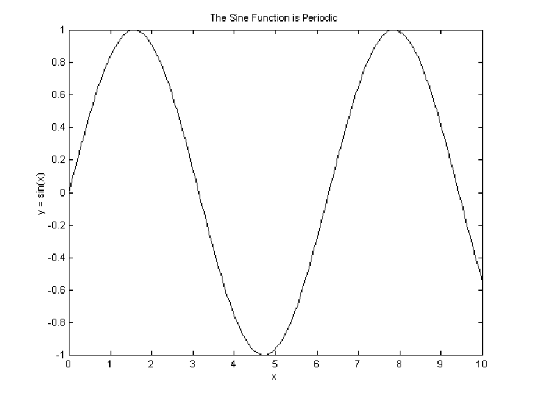
| x = linspace(0,10,200);
y = sin(x); plot(x,y) xlabel(`x') ylabel(`y = sin(x)') title(`The Sine Function is Periodic') |
| Use help to learn more about plot, xlabel, ylabel, and title. See also semilogx, semilogy, loglog, hist, bar, contour, and color. More general overviews of Matlab graphics can be obtained by using help to read about plotxy, plotxyz, and graphics. |

|
|
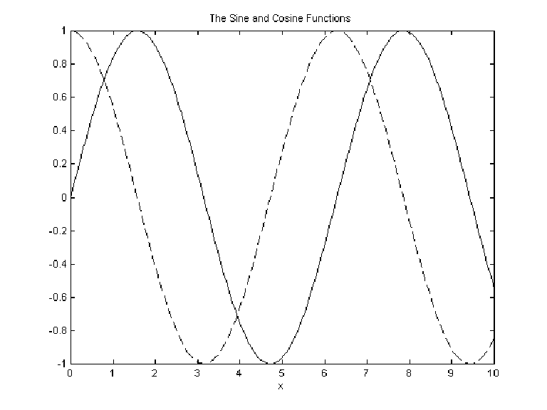
| x = linspace(0,10,200);
y = sin(x); z = cos(x); plot(x,y,x,z,'--') xlabel('x') title('The Sine and Cosine Functions') |
| Use help to learn more about plot. |
|
|
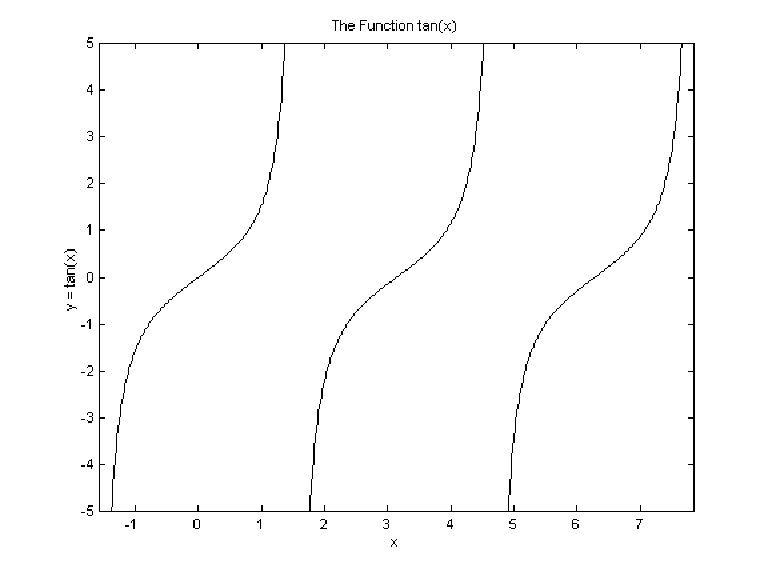
| x = linspace(-pi/2,pi/2,200);
y = tan(x); plot(x,y,x+pi,y,'-',x+2*pi,y,'-') axis([-pi/2,2.5*pi,-5,5]) xlabel('x') ylabel('y = tan(x)') title('The Function tan(x)') |
| Use help to learn more about axis. |
|
|
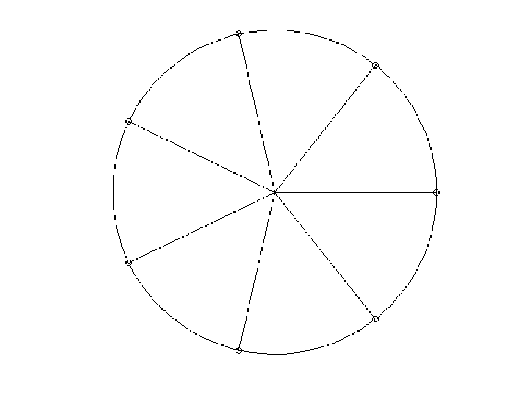
| a = linspace(0,2*pi);
plot(cos(a),sin(a)) axis('equal','off') a0 = linspace(0,2*pi,8); x0 = cos(a0); y0 = sin(a0); hold on for k=1:8 plot([0 x0(k)],[0,y0(k)],x0(k),y0(k),'o') end hold off |
| Use help to learn more about axis and hold. |
|
|
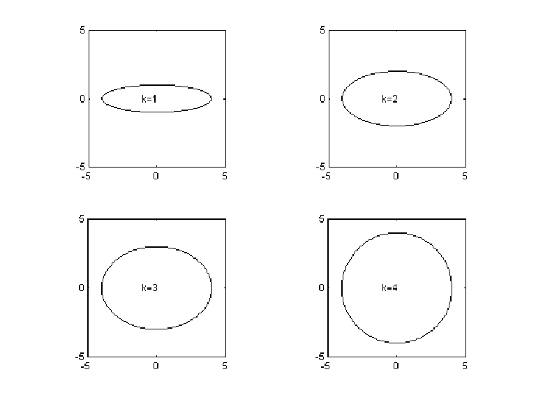
| a = linspace(0,2*pi,200);
c = cos(a); s = sin(a); for k=1:4 subplot(2,2,k) plot(4*c,k*s) axis('equal') axis([-5 5 -5 5]) text(-1,0,sprintf('k=%1d',k)) end |
| Use help to learn more about subplot, axis, and text. |
